For the Georgia Institute of Technology and its Nonlinear Systems class, my group performed analysis on a model for a small coaxial RC helicopter. The objectives of our study were to:
- Construct a model that accurately represented the dynamics of our system.
- Stabilize the system by finding and utilizing a Lyapunov function and feedback linearization.
- Create a simplified linear control system derived from the nonlinear dynamics of the model; then implement this control system on a real, commercially available RC helicopter.
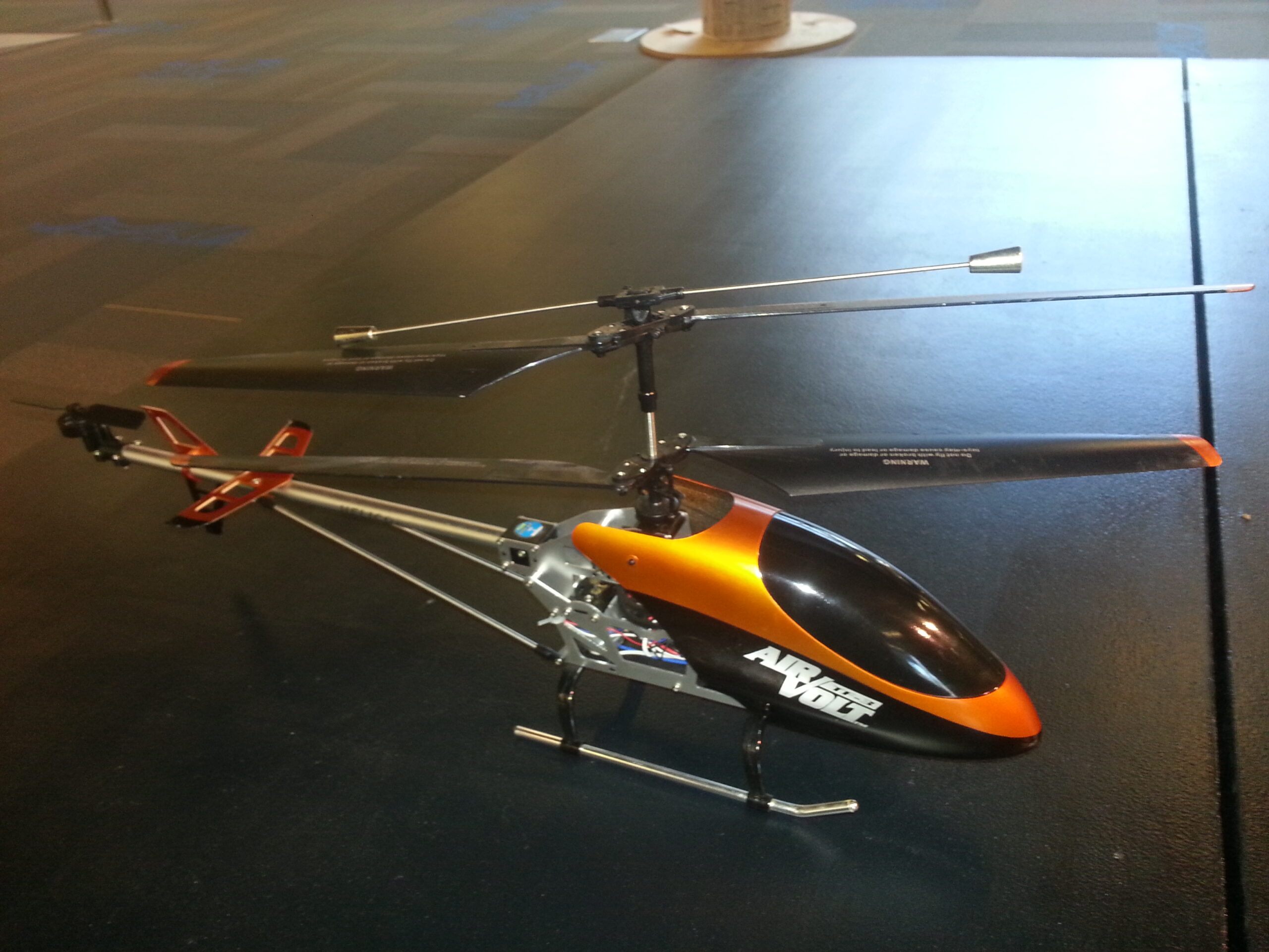
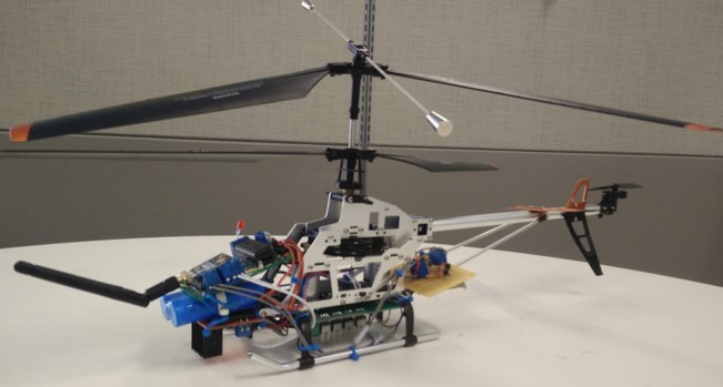
A standard RC helicopter with a burnt out controller was chosen as a starting point. A microcontroller (ARM Cortex M-0) was chosen to be the brain of the system. A LSM9DS0 IMU was chosen to be the acceleration and rotational sensor. The reference commands are to be transmitted wirelessly to the system by an XBee-PRO® 900HP transmitter.
The main rotors are powered by two motors which are to spin counter to each other. This is the central idea to the operation of coaxial helicopters. As a rotor rotates a torque is induced on the body of the helicopter which would cause the body to begin rotating. Since the rotors are spinning in opposite directions, their torque cancels out. By varying the difference in speed of the rotors, a small amount of torque can be allowed to cause desired rotation of the helicopter’s body.
The starting point of model development was based upon the work by D. Schafroth et al, titled “Modeling, system identification and robust control of a coaxial micro helicopter”. From there we developed the model, shown in Fig 1., to describe our system.
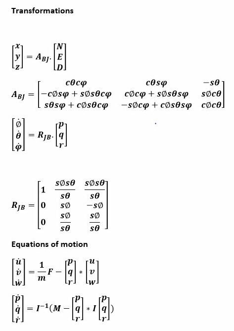
Here x,y,z and ϕ,θ,ψ are the position and the angular positions of the center of mass of the helicopter with respect to the origin. u, v, w and p,q,r are the linear and angular velocities in the x,y, and z directions. Ωdw and Ωup are the rotor speeds. In our model we assume the motor inputs to be equal.
The objective of the controller is to stabilize the helicopter in hover to a desired z value. During hover the system has freedom of angular velocity and acceleration about the z axis, or yaw.
The final step was to prepare our helicopter to perform our real world experiment. We converted our mathematical control system into a discrete version to run in our helicopter’s controller. The biggest problem we ran into was the weight of our new controller. The helicopter was only able to maintain flight for a few moments before succumbing to the weight and drifting downward. However for a few moments we where able to achieve a stable hover, and our control system performed quite well.
With more time and a larger budget, there are many things we could have done to improve the performance of our experiment. A more powerful helicopter with a longer lasting battery would have eliminated the weight issue and enabled us to perform longer tests. In the end we successfully confirmed our mathematical model with real world experimentation.
